Implications of Synergies in Asset Valuation and Arm’s Length Principle Compliance
It has been common to consider that market prices, and even the application of widely accepted “fair” asset valuation methods, are sufficient to comply with the arm’s length principle. However, this is not necessarily the case, as there are economic phenomena, such as synergies, that have peculiar implications.
Synergies imply that the interaction of assets, which can occur through their presence in the same organization, results in a joint value creation greater than the sum of the value creation of each asset individually, without interacting with each other.
In terms of an asset transaction, this could mean that the value contribution to the acquiring entity may not be the same as the value loss incurred by the selling entity.
Regarding the valuation of the asset in question, a widely accepted approach is the discounted cash flow method, where the main challenge is identifying the profits of the company attributable to the analyzed asset.
To simplify this point, the Shapley value tool can help us determine the profits that would “fairly” be attributable to a specific asset located in a company.
The Shapley value is a method of wealth distribution in cooperative game theory, assuming that all players collaborate in forming a grand coalition. It is a “fair” distribution in the sense that it is the only distribution with certain desirable properties (efficiency, asymmetry, linearity, and null player).
Given a group N (of n players) and a function υ : 2N → R with υ(∅) = 0, where ∅ denotes the empty set, the function v that assigns real actor subsets is called the characteristic function. The function v has the following meaning: if S is a coalition of players, then v(S), called the value of coalition S, describes the total sum of payments to the members of S that can be obtained through such cooperation.
According to the Shapley value, the amount that player i obtains during a coalition game (v, N) is:
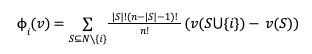
Where n is the total number of players, and the sum extends over all subsets of N that do not contain player i.
Example:
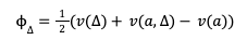
Let’s assume we have 3 players ({a, b, Δ}), where a represents the set of assets housed in A (excluding Δ) and b represents the set of assets housed in B, while Δ is a difficult-to-value asset.
Initially, asset Δ is owned by A, and its sale to B is being analyzed. Therefore, the estimation of the “fair” profit corresponding to asset Δ is:
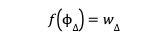
Assuming f(ϕ) = w, f: R → R is a function where ϕ is the annual profit of an asset and w is the present value of the asset.
The price of asset Δ would then be:
Arm’s Length Implications
However, A should not be willing to sell asset Δ for a price lower than f(v(a, Δ) – v(a)), as otherwise, it would not compensate for the loss of profits for A by ceasing to exploit asset Δ.
Therefore, if it were the case that v(Δ) < v(a, Δ) – v(a), which could indeed happen, w_Δ would not be arm’s length despite being a “fair” price, as it would not be a price that the owner of the asset would be willing to sell for.
Furthermore, if it were the case that v(a, Δ) – v(a) > v(b, Δ) – v(b), the contract curve between A and B would be empty. In other words, there would be no possible price for the transaction since any price would worsen the initial situation for either A, B, or both, which would not comply with the arm’s length principle.
The aforementioned leads us to reflect that while the priority of the transfer pricing framework is arm’s length compliance, it is common for the lack of information in the analysis to carry the risk of not being able to demonstrate the existence or find arm’s length prices. Nonetheless, market prices as well as theoretical “fair” prices can still be an acceptable alternative, especially in the practical application of transfer pricing analysis
JCG